How to Create a Timeline Filter in Excel
Excel is an essential tool for data analysis, and its advanced filtering features help users quickly analyze and visualize data. One such powerful feature is the Timeline Filter, which allows users to filter data dynamically based on time-related criteria. Unlike regular filters, a Timeline Filter is designed specifically for date fields, providing an intuitive slider to filter data by years, quarters, months, or days.
In this blog, we will explore what a Timeline Filter is, its benefits, and a step-by-step guide on how to create and use it effectively in Excel.
What is a Timeline Filter?
A Timeline Filter is a graphical filter that lets users filter a PivotTable or PivotChart dynamically based on time-based data. This feature is available in Excel 2013 and later versions. Unlike conventional filters, a Timeline Filter provides a scrollable and interactive slider, making it easy to filter data across different time periods without manually selecting date ranges.
Why Use a Timeline Filter?
Using a Timeline Filter offers several advantages, including:
- Easy Date-Based Filtering: Unlike drop-down filters, it allows users to select time periods with a simple drag of the slider.
- Multiple Time Groupings: You can filter data by Years, Quarters, Months, or Days, providing better control over data analysis.
- Interactive and User-Friendly: The filter is visually intuitive, making it easier to track trends over time.
- Improves Decision Making: By quickly analyzing specific time periods, users can make informed business decisions.
Step-by-Step Guide to Creating a Timeline Filter in Excel
To use a Timeline Filter, your dataset must include a date column. Follow these steps to insert and use a Timeline Filter in Excel.
Step 1: Prepare Your Data
Before inserting a Timeline Filter, ensure your dataset is structured properly. The dataset must contain at least one date-based column for the filter to work.
Here’s an example dataset of sales records:
| Date | Product | Sales |
|---|---|---|
| 01-Jan-23 | Item A | $500 |
| 15-Feb-23 | Item B | $700 |
| 10-Mar-23 | Item C | $650 |
| 25-Apr-23 | Item A | $800 |
| 12-May-23 | Item B | $900 |
| 05-Jun-23 | Item C | $750 |
| 20-Jul-23 | Item A | $850 |
| 15-Aug-23 | Item B | $950 |
| 30-Sep-23 | Item C | $1000 |
| 20-Oct-23 | Item A | $1100 |
| 10-Nov-23 | Item B | $1200 |
| 25-Dec-23 | Item C | $1300 |
Step 2: Create a PivotTable
A Timeline Filter only works with PivotTables. Follow these steps to create one:
- Select Your Data: Highlight the entire dataset including headers.
- Go to the Insert Tab: Click on the Insert tab in the ribbon.
- Click PivotTable: Select PivotTable from the menu.
- Choose the Data Source: Ensure the selected range includes all your data.
- Select Where to Place the PivotTable:
- Choose New Worksheet (recommended) or Existing Worksheet.
- Click OK.
Step 3: Add the Date Field to the PivotTable
Once the PivotTable is created:
- In the PivotTable Fields pane, drag the Date field into the Rows area.
- Drag the Sales field into the Values area.
- Your PivotTable should now display sales data grouped by date.
Step 4: Insert a Timeline Filter
Now that we have a working PivotTable, we can insert the Timeline Filter.
- Click anywhere inside the PivotTable.
- Navigate to the PivotTable Analyze tab.
- Click Insert Timeline.
- A pop-up will appear listing all date-based fields.
- Check the box for the Date field.
- Click OK.
You should now see a Timeline Filter added to your worksheet.
Step 5: Use the Timeline Filter
Once the Timeline Filter is inserted, you can begin filtering your PivotTable data dynamically.
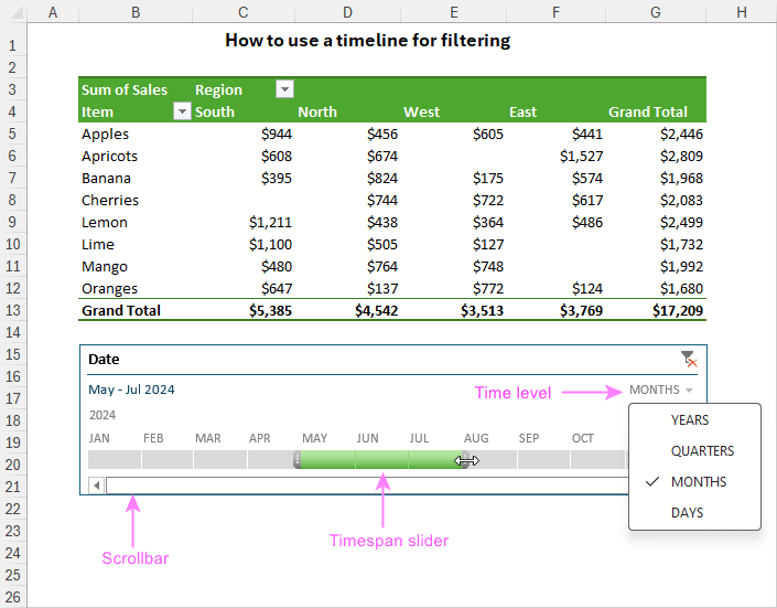
Using the Timeline Filter
- Select a Time Period: Click on the dropdown at the top-right of the Timeline Filter to choose between Years, Quarters, Months, or Days.
- Drag the Slider: Click and drag the slider to select a specific time range.
- Adjust the Selection: Click and extend or shrink the selected period.
- Clear the Filter: Click the Clear Filter button to reset the selection.
Customizing the Timeline Filter
Excel provides several ways to customize the Timeline Filter to improve usability and appearance.
1. Change the Timeline Style
- Click the Timeline Filter.
- Go to the Timeline Tools tab.
- Choose a different style under the Timeline Styles section.
2. Move and Resize the Timeline Filter
- Click and drag to move the Timeline Filter anywhere on the worksheet.
- Resize it by clicking and dragging the edges.
3. Formatting Options
- Click the Timeline, then go to Format Timeline options to change colors, font size, and layout.
Benefits of Using a Timeline Filter
- Improves Data Visualization: Allows easy tracking of data trends over time.
- Efficient Data Filtering: No need to manually filter date ranges in drop-down menus.
- Better Decision Making: Helps businesses analyze performance over different time frames quickly.
- User-Friendly: Even non-technical users can interact with data effortlessly.
Common Issues and Troubleshooting
1. Timeline Filter Option is Disabled
- Ensure your dataset contains a valid date field.
- The date column must be formatted as a Date and not as Text.
- The PivotTable must include the date field for the Timeline option to appear.
2. Timeline Filter Not Working Correctly
- Check if your PivotTable is refreshed (Right-click > Refresh).
- Ensure your date column is in a consistent format (e.g., DD/MM/YYYY or MM/DD/YYYY).
- Make sure you have selected the correct date range.
Conclusion
The Timeline Filter in Excel is a powerful tool for time-based data analysis, allowing users to easily filter and visualize data over different time periods. By following this step-by-step guide, you can insert and use a Timeline Filter effectively in Excel to improve your data analysis workflow.
Whether you’re tracking sales, analyzing financial data, or reviewing project timelines, using a Timeline Filter makes data exploration faster and more interactive. Try it in your Excel workbook today and experience the benefits!